Hyperparameter Tuning for K Nearest Neighbors

Sunday. March 10, 2019

Introduction

KNN is a supervised learning algorithm with the intended goal of classifying a new instance by comparing it to the training instances. Specifically, the value of the target function for a new query is estimated from the known value(s) of nearest training examples. Consider a set of training instances \((x,y)\), the goal is to learn a function \(f: X \rightarrow Y\) such that \(f(x)\) can correctly classify new instances correctly with high confidence.

Two important properties of KNN:

Instanced-Based
Non-Parametric

Instance-based Learning

In instanced-based classification, no model is learned the stored instances represent the knowledge. Training instances are searched for an instance that has the most similarities or closely resembles the new instance. A similar real-world example is that of rote learning. In the context of machine learning it can be used to describe a simple learning pattern, although it does not involve repetition (as per the usual definition of rote learning). Consider a machine that is programmed to keep a history of calculations and compare new input against its history of inputs and outputs, retrieving the stored output if present. This was the approach used by Arthur Samuel in 1959 for various rote learning mechanisms by which a program could become better at computer checkers. His work used an early version of what is now called alpha-beta pruning.

In machine learning instance-based learning provides an alternative to parametric models. Such non-parametric models construct its predictions directly from the training instances themselves instead of performing explicit generalizations. As a result, the learning amounts to storing the data.

Non-Parametric

Non-parametric models can be used with arbitrary distributions and without the assumption that the form of the underlying density is known. There are two types of nonparametric methods:

Estimating class conditional densities, P (X \(\|\) \(\theta\))
Bypass class-conditional density estimation and directly estimate the a-posterior

Additionally, KNN makes no explicit assumptions regarding the underlying distribution of the data or about the form of \(f\), the hypothesis.

Distance Metrics

The value of the target function for a new test instance is estimated from the known value of the nearest training example(s). The nearest neighbor(s) are found using a distance measure or metric. The distance metric, d(x^{(a)},x^{(b)}), typically used (and for the rest of this article) is defined to be Euclidean. Common distance metrics include:

Euclidean: \(d(x^{(a)},x^{(b)}) = \sqrt{\sum_{i=1}^{d}\|(x^{(a)}_i - x^{(b)}_i)}\|\)
Manhattan: \(d(x^{(a)},x^{(b)}) = \sum_{i=1}^{d}\| x^{(a)}_i - x^{(b)}_i \|\)
Minkowski: \(d(x^{(a)},x^{(b)}) = \sqrt[q]{\sum_{i=1}^{d}\| x^{(a)}_i - x^{(b)}_i \|^{q}}\)

There are many other distance metrics (Tanimoto, Jaccard, Cosine) but they should be chosen based on the properties of your data.

Nearest Neighbor

The nearest neighbor algorithm is simply a case of KNN where \(k=1\). An important property of the nearest neighbor algorithm for binary classification is that it is not more than twice the Bayesian error rate.

Find k examples \({x^{(i)},t^{(i)}}\) (from the stored training set) closest to the test instance x that is:
\[x^{*} = \underset{x_{i}\in TrainSet}{\arg\min} \| x^{(a)} - x^{(b)} \|_2\]
Output:
\[y = t^{*}\]

K Nearest Neighbors

KNN is an extension of NN, where we find K nearest neighbors and return the majority vote of their labels. K yields smoother predictions, since we average more data.

Find k examples \({x^{(i)},t^{(i)}}\) closest to the test instance x
Classification output is majority class
\[y = \underset{t_{i}\in TrainSet}{\arg\max} \| x^{(a)} - x^{(b)} \|_2\]

How do we choose k?

A good question to consider is how to choose k, larger k may lead to better performance but if we set k too large we may end up looking at training points that are far away from the new test instance. One possible solution is to use cross-validation to find the optimal k.

Rule of thumb: \(k< \sqrt{n}\), where n is the number of training instances.

Parameter Tuning with Cross Validation

Here we will discuss a method that can be used to find the optimal k value. Cross validation is used to estimate the test error associated with a learning method in order to evalute its performance, or to select the appropriate level of flexibility. The training set is divided into t groups or folds (typically k but we use k for number of neighbors) of approximately equal size. The first fold is the validation set and the remaining \(t - 1\) folds is the training set the method is fit on. The misclassification error is computed on the validation set. This is repeated for all t choices of the validation set. For each choice of k, find the average error across validation sets. Choose the value of k with the lowest error.

# loading the digits data set.
digits = load_digits()

print ("We have", digits.data.shape[0], "data points in total.")
print ("Each data point has", digits.data.shape[1], "features. In fact, each instance is an 8x8 picture of a digit.")
print ("Each digit's target/class/label is one of", list(set(digits.target)))

# We want to turn the problem into a binary classification one.
# Therefore, from the data set, we only pick those digits whose label is either 0 or 1
X = digits.data[(digits.target==0)|(digits.target==1)]
Y = digits.target[(digits.target==0)|(digits.target==1)]
print ("The reamining number of data points is", X.shape[0])

We have 1797 data points in total.
Each data point has 64 features. In fact, each instance is an 8x8 picture of a digit.
Each digit's target/class/label is one of [0, 1, 2, 3, 4, 5, 6, 7, 8, 9]
The reamining number of data points is 360

def show_some_digits(X, Y):
    plt.figure(figsize=(20,8))
    for index, (image, label) in enumerate(zip(X[0:30], Y[0:30])):
        plt.subplot(3, 10, index + 1)
        plt.imshow(np.reshape(image, (8,8)), cmap=plt.cm.gray)
        plt.title('Target Label: %i\n' % label, fontsize = 10)
    return

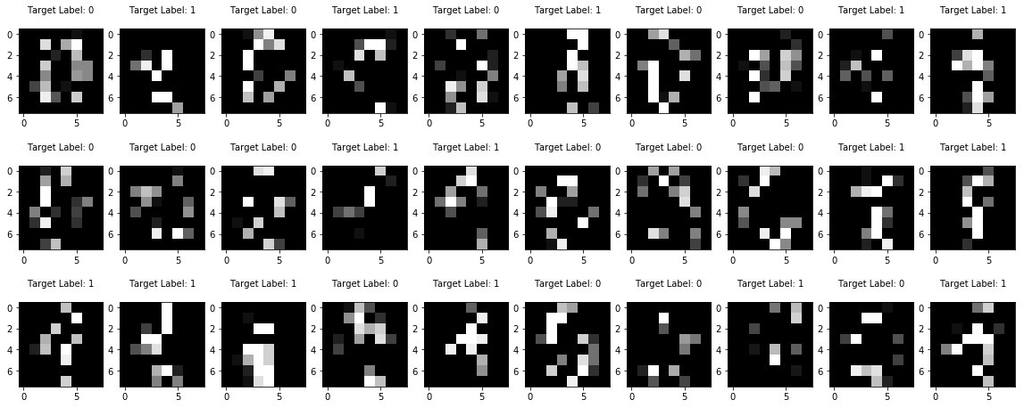
def blurr_digit (X, drop_probability):
# This is how we create the noisy data set
    return np.multiply(X, np.random.choice([0, 1], size=(360,64), p=[drop_probability, 1 - drop_probability]))


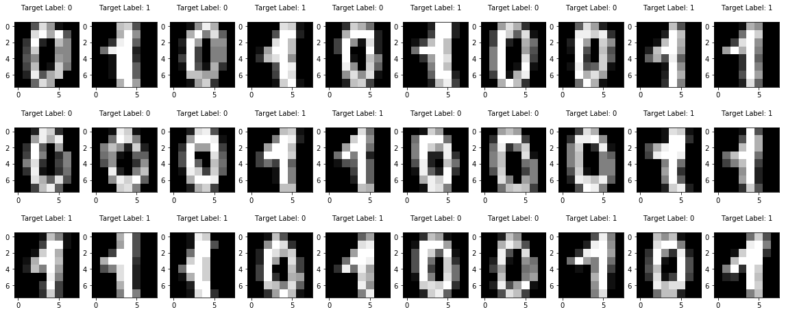
print ("Hear are some of the original digits (first three rows)...and then their noisy versions")
show_some_digits(X, Y)
plt.show()
X_noisy = blurr_digit (X, 0.6)
show_some_digits(X_noisy, Y)
plt.show()

Hear are some of the original digits (first three rows)...and then their noisy versions

png

SkleanKNN = KNeighborsClassifier(n_neighbors=8)

cvScores = []
kList = list(range(1,21))

for k in kList:
    KNN = KNeighborsClassifier(n_neighbors=k)
    scores = cross_val_score(KNN, X_noisy, Y, cv=10,scoring="accuracy")
    cvScores.append(scores.mean())

MSE = [1 - x for x in cvScores]
optimal_k = kList[MSE.index(min(MSE))]
print ("The optimal number of neighbors is %d" % optimal_k)
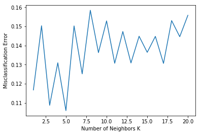
# plot misclassification error vs k
plt.plot(kList, MSE)
plt.xlabel('Number of Neighbors K')
plt.ylabel('Misclassification Error')
plt.show() 

The optimal number of neighbors is 5

Markdown Image